 WonksAnonymous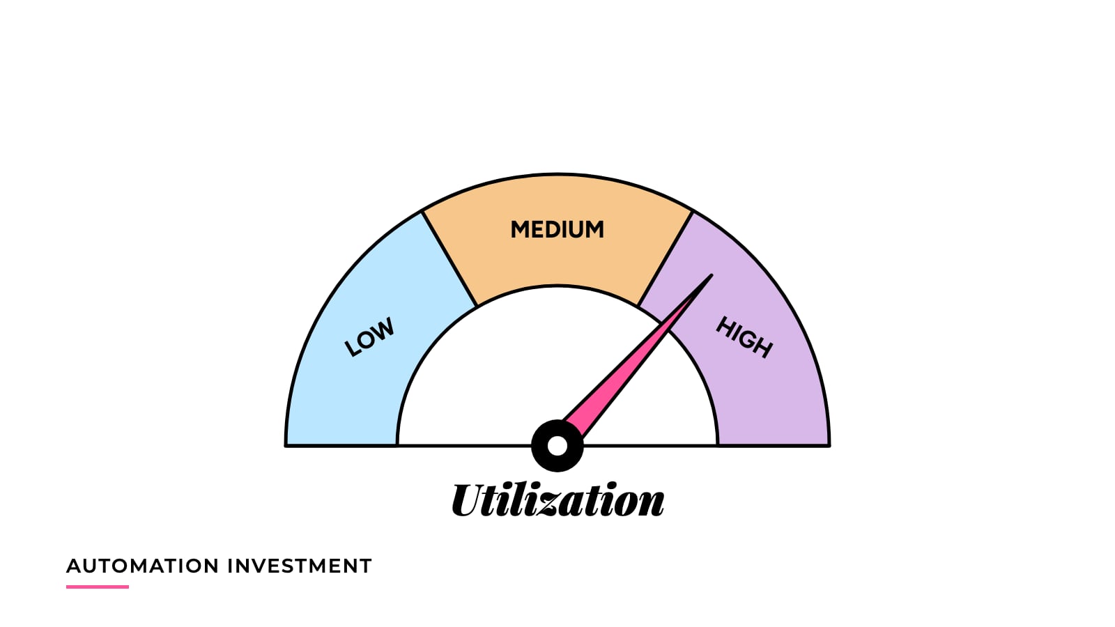
How Equipment Utilization Changes Automation Payback
Low, medium and high utilization scenarios for one $60,000 automation case, with a sensitivity check and a break-even hours formula.
A machine saves money only when it runs on real orders. The same equipment, bought at the same price, can pay back in 16 months in one plant and in nearly seven years in another (in this example), and the main difference is how many productive hours it works.
This article runs one investment through three utilization scenarios, checks which input matters most, and shows how to calculate the hours you need to hit a payback target. It uses the same $60,000 investment as the payback, ROI and TCO article.
The model
The simple payback formula assumes a steady annual benefit. Here the benefit is tied to productive hours, because most savings (labor not paid, material not wasted, orders filled in-house) occur only while the machine is producing.
B = (net cash benefit per productive hour x productive hours per year)
    - fixed annual cash costs

Payback (years) = I / B, only when B > 0
Payback (months) = payback in years x 12
“Net cash benefit per productive hour” is the cash saved or earned per hour of running, after the variable costs of running. “Fixed annual cash costs” occur whether or not the machine runs, for example a service contract. When B is zero or negative, there is no positive payback under these inputs and this simplified model.
Inputs and scenarios
Illustrative numbers, not a quote, benchmark or customer result.
| Input | Value |
|---|---|
| Installed investment (I) | $60,000 |
| Net cash benefit per productive hour | $12 |
| Fixed annual cash costs | $3,000 |
Three scenarios for productive hours per year. The shift mapping is approximate: a single shift of 8 hours over about 250 working days is 2,000 hours if the machine runs the whole time, so 1,000 hours is roughly half a shift, 2,000 is roughly one full shift and 4,000 is roughly two shifts. Real plants lose hours to changeovers and stoppages, so treat the mapping as a rough guide only.
| Scenario | Productive hours per year | Net benefit (hours x $12) | Fixed costs | B | Payback (years) | Payback (months) |
|---|---|---|---|---|---|---|
| Low | 1,000 | $12,000 | $3,000 | $9,000 | 6.67 | about 80 |
| Medium | 2,000 | $24,000 | $3,000 | $21,000 | 2.86 | about 34 |
| High | 4,000 | $48,000 | $3,000 | $45,000 | 1.33 | 16 |
Check the arithmetic: 60,000 / 9,000 = 6.67 years (x 12 = 80 months); 60,000 / 21,000 = 2.86 years (x 12 = 34.3 months); 60,000 / 45,000 = 1.33 years (x 12 = 16 months).
Why the relationship is not linear
Doubling hours from 1,000 to 2,000 does not halve the payback in a simple way. B rises from $9,000 to $21,000, which is a factor of 2.33, because the $3,000 fixed cost is paid once regardless. Payback falls from 80 to 34 months. Doubling again to 4,000 hours lifts B to $45,000 (a factor of 2.14) and payback falls to 16 months.
Fixed costs also set a floor. At $12 per hour and $3,000 fixed, the machine must run 3,000 / 12 = 250 hours a year just to cover the fixed cost. Below that, B is negative and there is no payback.
At low hours, the fixed costs consume a large share of the gross benefit (3,000 of 12,000, or 25%, in the low case, against 6.25% in the high case). That is why the low scenario is worse than a straight-line reading of hours would suggest.
What pushes productive hours down
Several things reduce productive hours below what the shift schedule suggests:
- Order volume. If orders fill half a shift, the machine runs half a shift. Capacity does not create demand.
- Number of shifts. A machine staffed for one shift cannot reach the two-shift scenario without added labor cost, which belongs in B.
- Changeovers. Every product switch removes minutes or hours from production. Frequent small batches multiply this loss.
- Unplanned downtime. Stoppages cut hours and can leave orders late.
- Waiting on upstream or downstream. A machine that waits for material or for the next station is not productive, however fast its rated speed. See why faster machines do not always increase line output and cost per good pack for how to count good output instead of nameplate speed.
Sensitivity check
Take the medium scenario (2,000 hours, baseline payback 2.86 years, about 34 months) and change one input at a time.
| Change | New B | New I | Payback (years) | Payback (months) | Change vs. baseline |
|---|---|---|---|---|---|
| Baseline | $21,000 | $60,000 | 2.86 | about 34 | none |
| Net benefit per hour 25% lower ($9) | $15,000 | $60,000 | 4.00 | 48 | about 14 months longer |
| Installed cost 20% higher ($72,000) | $21,000 | $72,000 | 3.43 | about 41 | about 7 months longer |
The arithmetic: at $9 per hour, B = 9 x 2,000 - 3,000 = 15,000, and 60,000 / 15,000 = 4.00 years (48 months). At 20% higher cost, I = 60,000 x 1.2 = 72,000, and 72,000 / 21,000 = 3.43 years (41.1 months).
In this example, a 25% shortfall in hourly benefit hurts about twice as much as a 20% cost overrun. Verify the hourly benefit and the productive hours first. They drive B, and B is the denominator. An error in either also moves payback further than the same-sized error in installed cost, which can be checked against a quote and a scope list. See the true installed cost of packaging automation for that check.
A 25% drop in hours has a similar effect to a 25% drop in hourly benefit, since the two multiply. Check both.
Break-even utilization
You can reverse the model: given a target payback, how many productive hours are needed?
Hours needed = (I / target years + fixed annual costs) / net benefit per hour
Example: a 3-year target with the same inputs. I / target years = 60,000 / 3 = 20,000 per year. Add fixed costs: 20,000 + 3,000 = 23,000. Divide by $12: 23,000 / 12 = 1,917 productive hours per year (rounded up).
Check: 1,917 x 12 = 23,004; minus 3,000 = 20,004; 60,000 / 20,004 = 3.00 years. A 2-year target would need (30,000 + 3,000) / 12 = 2,750 hours. If your realistic hours fall short of the number the formula gives, the target is not met under these inputs.
Estimate your own utilization
- Use order history, not capacity. Count the hours that produced paid output last year, not the hours the machine could have run.
- Subtract changeovers and downtime. Use logged records where they exist. If they do not, estimate conservatively and label the estimate.
- Separate committed orders from hoped-for orders. Run the model on committed volume first, then show the hoped-for volume as an upside scenario.
- Check that the cash benefit holds at that volume. If the saving is labor, confirm that wages actually stop. See labor savings versus redeployment.
When current volume is well below break-even hours, the model may say the machine is not justified yet, or that a smaller or semi-automatic solution would fit better. That is a legitimate result.
Keep reading
- Automation Payback, ROI and TCO: What Each Metric Tells You: defines the three metrics and runs the same $60,000 case through each.
- The True Installed Cost of Packaging Automation: lists the costs that belong in I beyond the machine price.
- Labor Savings Versus Redeployment: Avoiding False Payback Claims: separates cash savings from freed hours before you set the hourly benefit.
Assumptions and limits
- Net benefit per productive hour is treated as constant. In practice it can change with product mix, scrap rates and order size.
- The model ignores taxes, financing, the time value of money, ramp-up, residual value and useful life. It is a simple payback, not NPV or IRR.
- The shift-to-hours mapping is approximate and assumes about 250 working days of 8 hours.
- All inputs are invented for illustration. Replace them with verified figures from your own records.
- The model supports comparison and does not replace financial, legal, safety or engineering review. Calculators are in preparation and will be published only after testing.